Last time, I finished working on my Alaska map with political boundaries and shading in place, and the major rivers and lakes depicted. This time, I’m going to use some more Natural Earth data to add more information to the map.

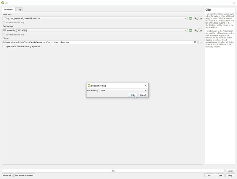
The first thing I want is some towns and villages, so I download the Natural Earth “Populated Places” vector dataset from the “Cultural” section of the download page, unzip it into my default directory, and clip it down to just my area of interest, as I’ve described in previous posts. But there’s an important consideration during the clipping process, this time. Northern Iñupiat placenames use a special “dotted g” (ġ) character, which I’ll lose if I don’t make sure that the clipped file is saved with an appropriate character set. So I process this one individually, which lets me set the character set of the clipped file. Having gone through Vector>Geoprocessing Tools>Clip…, I set “Input layer” to ne_10m_populate_places.shp (the original Natural Earth file), and “Overlay layer” to the clipping mask I saved in Part 1. Then I click on the […] button to the right of the “Clipped” text box, choose “Save to File…” and call my clipped file alaska_ne_10m_populated_places.shp, consistent with my other clipped files. But then I click on […] again, and select “Change File Encoding” which will let me choose from a huge array of potential character sets. I make sure to set this to UTF-8, which will retain any special Inuit characters in the original dataset, and then click the Run button. After all that, I can load the shape file as a new vector layer, and start formatting the way towns and other settlements are displayed.

There are a lot of very small settlements in Alaska, and I want to give some indication of the largest population centres. So I double-click on my alaska_ne_10m_populate_places layer to bring up the Layer Properties dialogue box, and set up some rule-based symbology, as previously described. After poking around in the very large number of data fields supplied by Natural Earth, I establish that POP_MAX contains the numbers I want, and set up two sets of symbols—a large marker that corresponds to populated places that match the rule:

“POP_MAX” >20000

and a smaller marker for:

“POP_MAX” <=20000

To label these points I can just use the NAME field, but I’m going to do something more complicated. Natural Earth stores some alternative placenames in a field called NAMEPAR, so I want to set up a rule-based label that will add the alternative name in brackets if one exists—so I can display Iñupiat and English placenames side by side, for historical interest.

I test for the absence of an alternative name with the rule:

“NAMEPAR” is NULL

If this is true, I just label with the NAME field. But then I set up the handy rule ELSE, which will be true only if there’s something worth printing in the NAMEPAR field.

Now I need to find a way to combine the contents of two dataset fields (NAME and NAMEPAR), along with some additional text, into a single label. In the Edit Rule window, there’s a button labelled with a little epsilon (ε) next to the “text box in which you enter the name of the data field to be used for labels”Value” text box for Labels. I’ve marked it with the mouse cursor in the screenshot below:

If I click on this, I can combine fields into one label, using QGIS’s string concatenation operator “||”. This is available on one of a row of buttons featuring common operators (additions, subtraction, etc) at lower left of the Expression Dialog window, or you can type it from the keyboard by entering the “vertical bar” character twice. Again, I’ve marked the button with the mouse cursor, below:

As you can see from my screenshots, my method of combining fields looks like this:

“NAME” || ‘ (‘ || “NAMEPAR” || ‘)’

Disappointingly, it turns out there’s only one place on my map that has an alternative name listed by Natural Earth. Here it is, showing the effect of my string-concatenation rule (as well as showing that I’ve properly carried over the dotted-g character into my clipped dataset):

Here’s a screenshot of the label rules in final form:

But there’s a problem. Despite all this effort, when I plot my map some of my populated places don’t have labels. (Notice, for instance, the two unlabelled settlements on the Mackenzie River between Fort McPherson and Norman Wells.)

It seems that my label text is fighting for space with some of the other features on the map, particularly rivers. I find I can fix this problem by editing the “Placement” option for label text. Right at the bottom of this set of options, there’s a check-box labelled “Features act as obstacles”. Turning this off makes QGIS more willing to overwrite other map features. I disable this both for populated places and for rivers, and QGIS then manages to accommodate (almost) all my labels. Again, the location of the relevant check-box is marked with the mouse cursor, below:

To finish off this post, I’ll add roads and railways, which are available as cultural vector datasets. Each comes with a North American supplement, and the supplementary roads dataset is very useful for showing the extensive unpaved Alaskan road system. I download the files, unzip them, clip them, and add them as new layers.

Adding railways is easy—there’s even a nice pre-formatted “railway” symbol in the Layer Properties window, though I tweaked the thickness of the line and width of the crossbars for visibility.

The two road datasets are complementary, to some extent. The main file is better at showing ferry routes (which I don’t particularly want). The North American supplement is better for minor roads (which I do want). So I went with just the supplemental dataset for this project. It stores a useful road classification in a field called type. So I set up Symbology rules to mark Primary and Secondary roads with a thick red line, minor paved roads with a thin red line, and unpaved roads with a black dashed line, like this:

And here’s the result:

Nearly there. Next time, I’ll add some additional detail, including importing a dataset from a source other than Natural Earth.